Tutorial 1: Discriminate the correct fold of proteins
To check the example of this tutorial, click here.
In this tutorial we will work with the structure of the Cysteine synthase A from E.coli; obtained from the CASP12 dataset as target T0861. We will test a dataset including a native structure, a near native model and a wrong model. The first step is to select the "protein folds" option, select a distance for the contact definition and submit a compressed file with the structures under study. In this tutorial we will work with the "CB-CB distance < 12A" option. To access the results page click in “run example”.
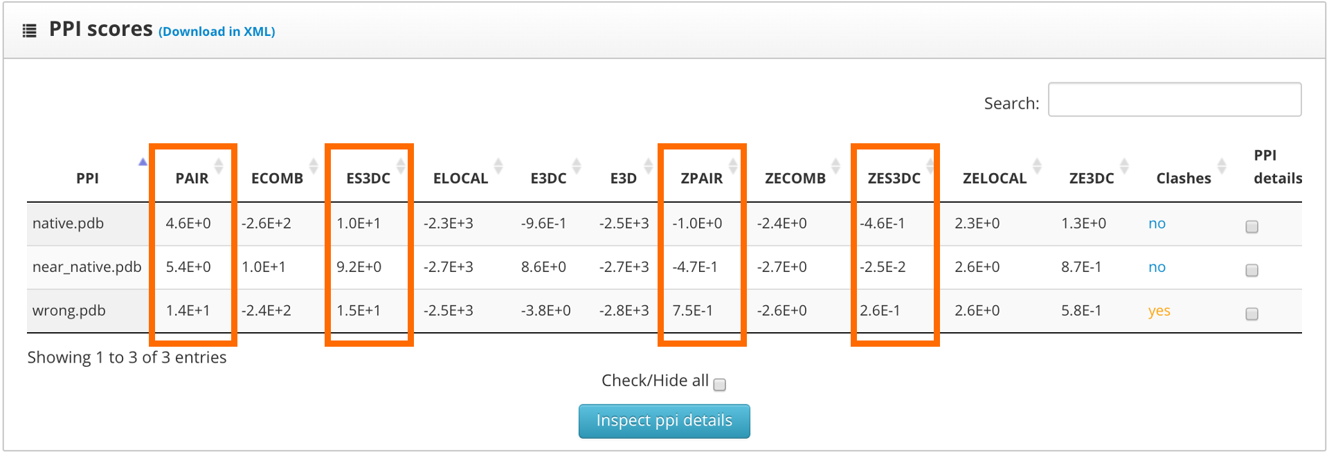
The results page shows the global scores for the input structures. Check the PAIR, ZPAIR, ES3DC and ZES3DC scores; you can see them highlighted in here:
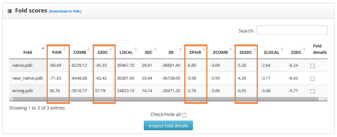
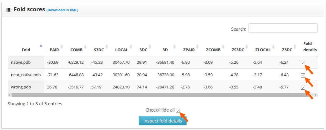
To identify the best folded structures we check for the lowest score in the previously mentioned scoring functions. We see that the native structure has the lowest scores, followed by the near native model. To perform a more detailed analysis we select the "fold details" option and click into the "inspect fold details" button.
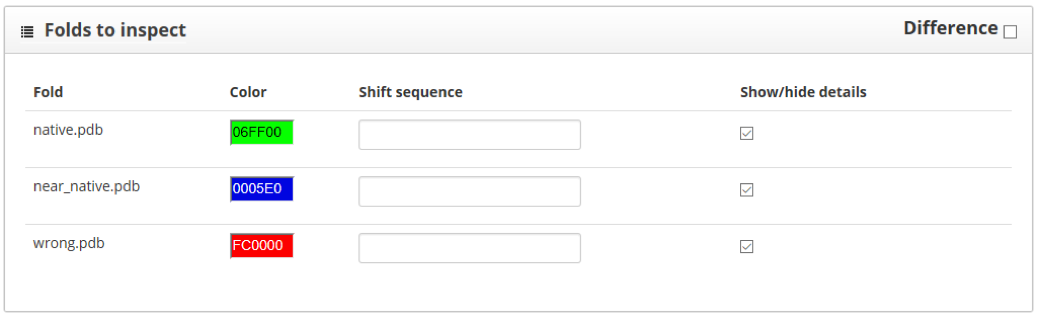
Here we find two sections: "folds to inspect" and "residue scores". The "folds to inspect" section allows the assignment of a color to each structure, the shift of a protein sequence or the plotting of score differences between structures.
The "residue scores" section shows the scores along the protein sequence, represented in the x axis of the plot. We can smooth the plot curve by increasing the "Sliding window" value, this will make it easier to understand. Here we see the native structure in green, the near native one in blue and the wrong model in red:
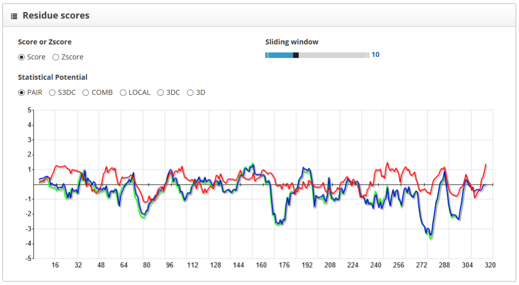
For the PAIR scoring function, we see that the structure with lowest scores is the native one, followed closely by the near native model. Another way to visualize the difference between structures is to use the "difference" tool in the "folds to inspect" section. By doing so and setting the native structure as reference, we clearly see the differences between models in comparison with the native structure:
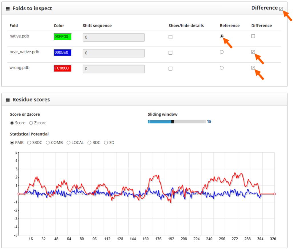
As the score profile for the near-native model has lower values along the protein sequence, we can differentiate it from wrong models.
Tutorial 2: Predict the stability of mutant proteins
To check the example of this tutorial, click here.
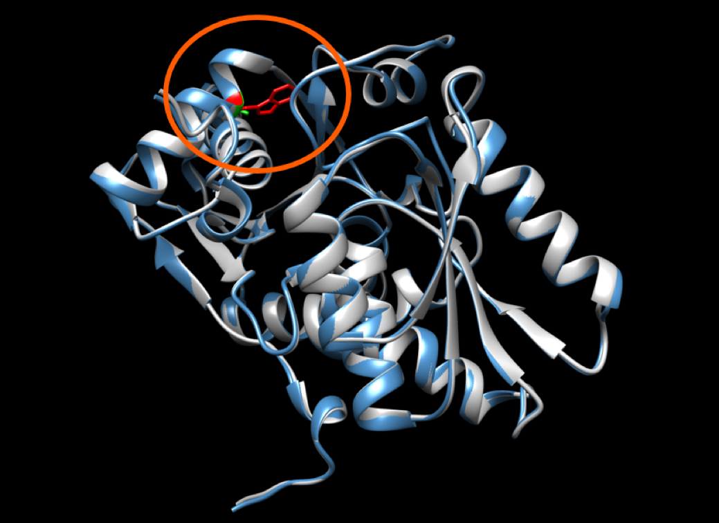
In this tutorial we will work with the structure of the Cysteine synthase A from E.coli; obtained from the CASP12 dataset as target T0861. We have obtained an homology model of this structure that contains a mutation using modeller. This mutation is a substitution of an alanine by a triptophan in position 255. You can see the superimposition of the two structures in the following image with the wild type and mutated residues highlighted in green and red, respectively:
The first step is to select the protein folds option, select a distance for the contact definition and submit a compressed file with the structures under study. In this tutorial we will work with the "CB-CB distance < 12A" option. To access the results page click in "run example".
The results page shows the global scores for the input structures. Check the PAIR, ZPAIR, ES3DC and ZES3DC scores; you can see them highlighted in here:
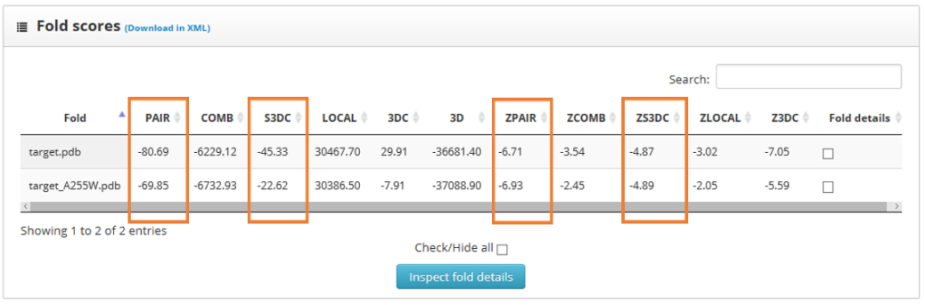
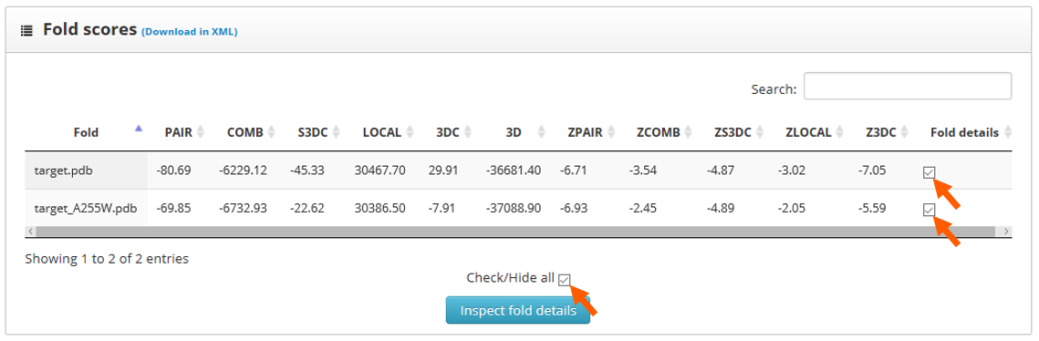
To identify the best folded structures we check for the lowest score in the previously mentioned scoring functions. We see that the wild type structure has the lowest scores. To perform a more detailed analysis we select the "fold details" option and click into the "inspect fold details" button.
Here we find two sections: "folds to inspect" and "residue scores". The "folds to inspect" section allows the assignment of a color to each structure, the shift of a protein sequence or the plotting of score differences between structures.
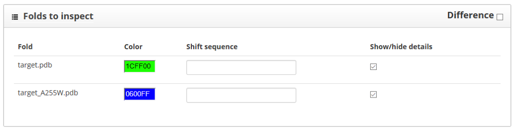
The "residue scores" section shows the scores along the protein sequence, represented in the x axis of the plot. It is better to keep the sliding window value set to 1, so we can see more clearly score changes happening because one single amino acid. Here we see the wild type in green and the mutant in blue:
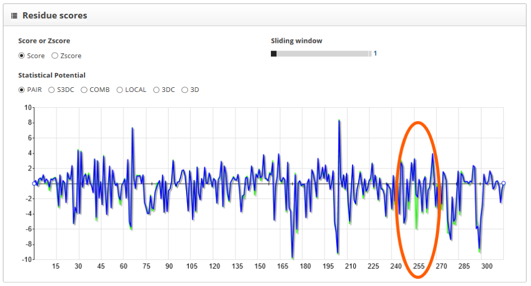
For the PAIR scoring function we see that the wild type protein has lower values on position 255. Another way to visualize the difference between structures is to use the "difference" tool in the "folds to inspect" section. By doing so and setting the wild type protein as reference, we clearly see the effect of the mutation in the scoring profile:
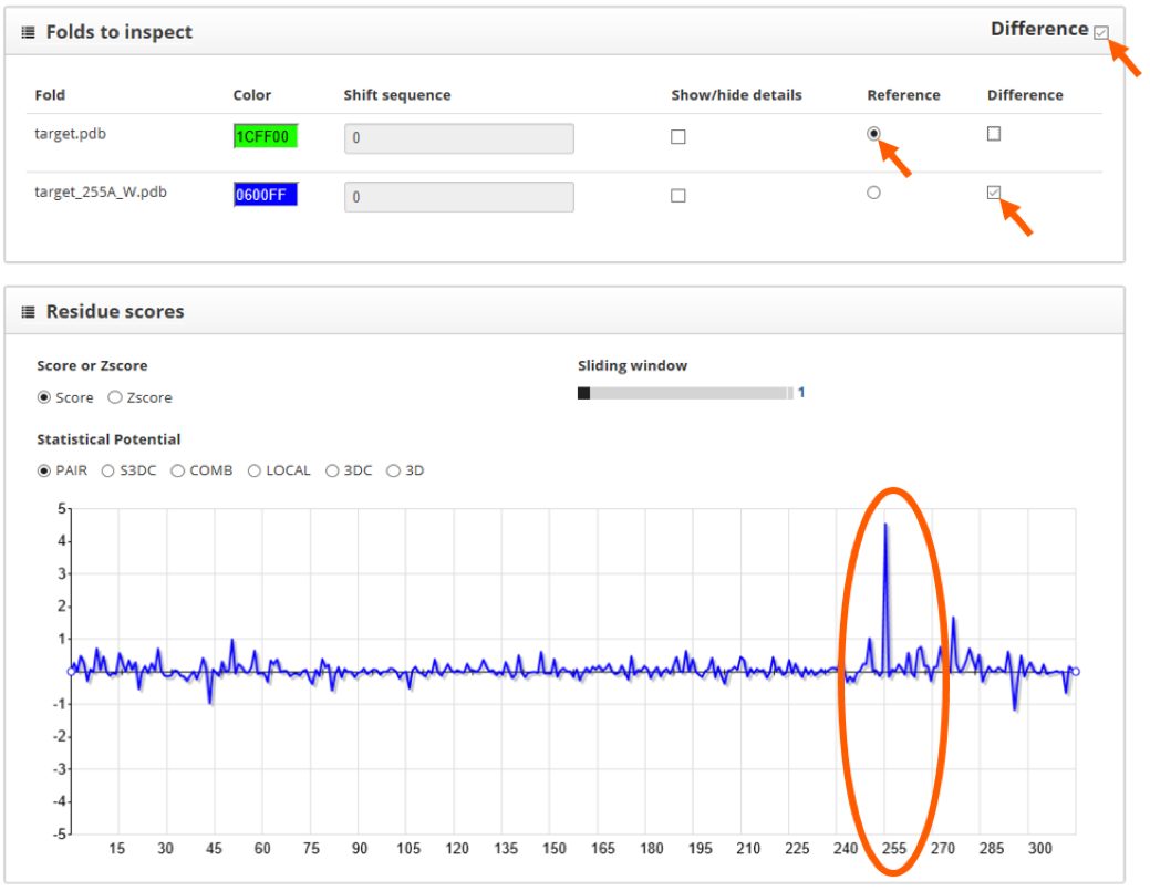
Since this mutation increases the score of the wild type protein, we conclude that the effect of this mutation is to destabilize the protein fold.
Tutorial 3: Identify near native docking poses
To check the example of this tutorial, click here.
In this tutorial we will work with the structure of docking solutions obtained from the CAPRI scoring dataset, in particular with the target 53. We will test a dataset including a native structure, a near native pose and a wrong pose. The first step is to select the Protein-protein interactions option, select a distance for the contact definition and submit a compressed file with the structures under study. In this tutorial we will work with the "CB-CB distance < 12A" option. To access the results page click in "run example".
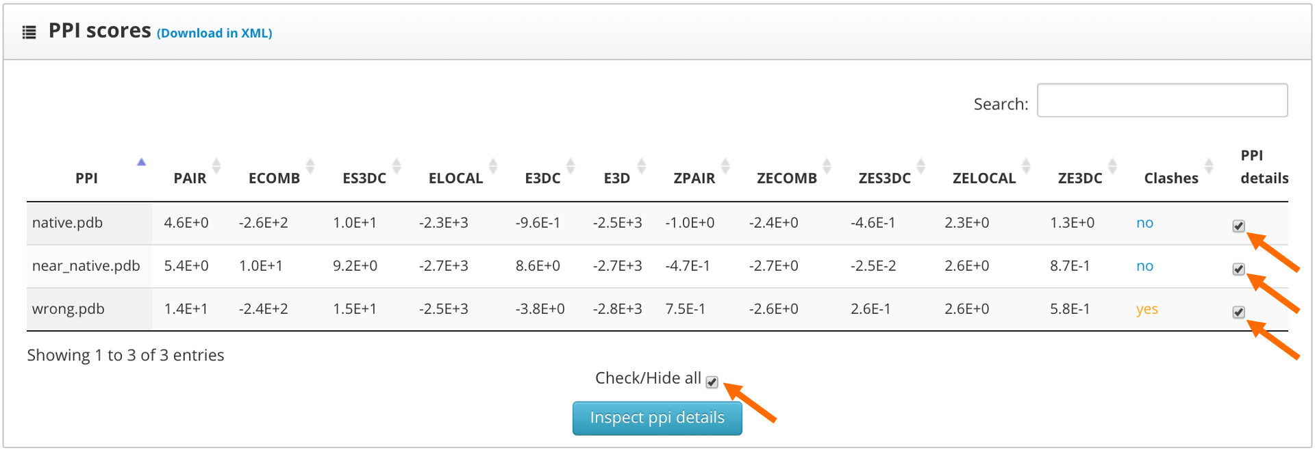
The results page shows the global scores for the input structures. Check the PAIR, ZPAIR, ES3DC and ZES3DC scores; you can see them highlighted in here:
To identify the best folded structures we check for the lowest score in the previously mentioned scoring functions. We see that the native structure has the lowest scores, followed by the near native model. To perform a more detailed analysis we select the "fold details" option and click into the "inspect fold details" button.
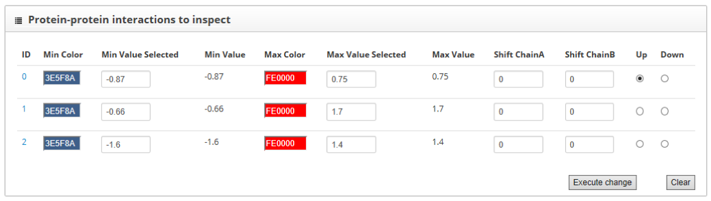
Here we find two sections: "Protein-protein interactions to inspect" and "residue scores". The "Protein-protein to inspect" section allows the assignment of colors to high and low scoring residues. It also allows to shift the protein sequences and to assign the up or down label to each one of the proteins.
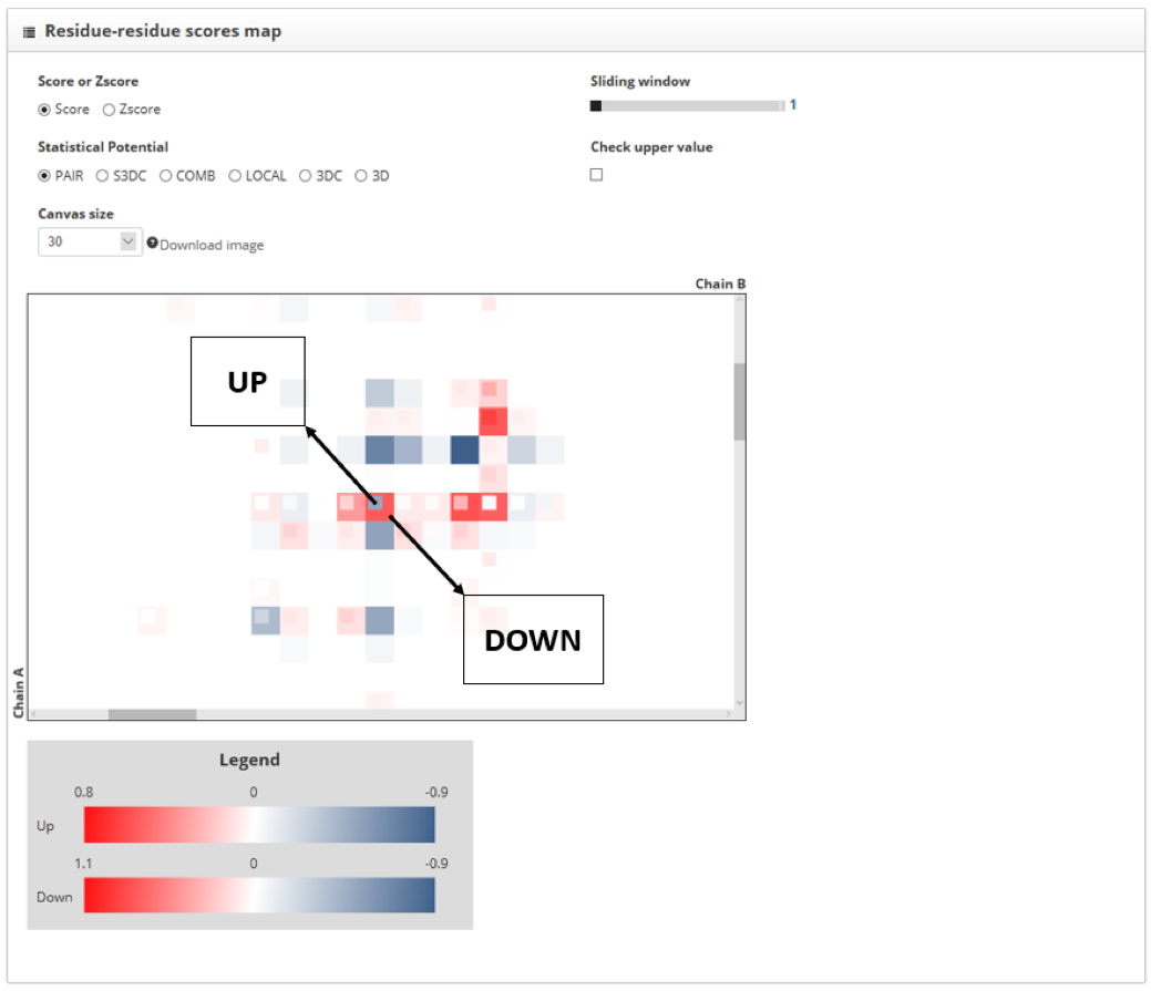
The "residue-residue scores map" section shows the representation from each of the interacting proteins in a different axis. Contacts between the two chains are represented as color dots. The color of these points is informative of whether the contact increases or decreases the stability of the interaction. We can smooth the score map using the "sliding window" tool and increase the size of the map using the "canvas size" option. Besides, the "check upper value" shows the scores for each of the residues of the "up" labeled structure, within the score map.
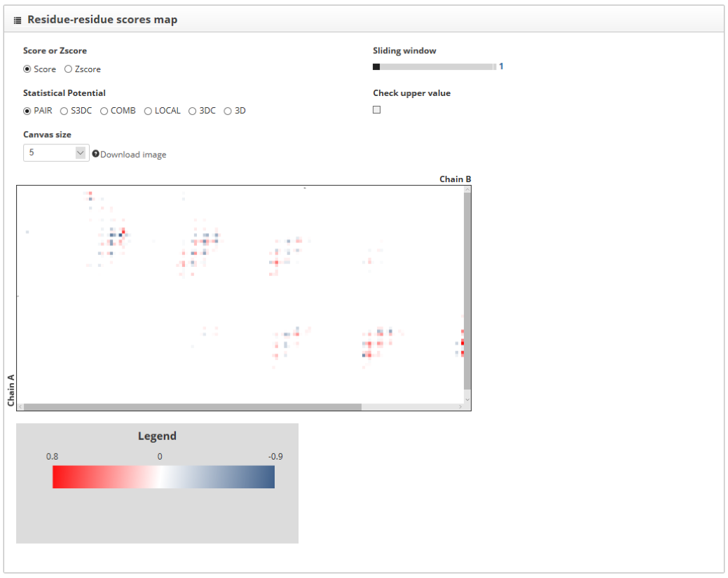
To compare two PPIs we must assign to them the up or down label in the "Protein-protein interaction to inspect" section. If we increase the size of the score map we will see that the protein contacts for the “up” structure are represented with small squares, while the "down" structure ones are represented with big hollow squares. When the same contact is found in both structures, the two squares that represent them fit.

The color of the square is telling us which contacts increase PPI stability and which do not. The color corresponding with the "min color" label in the "protein-protein interactions to inspect" indicates low scores and high stability, while the one corresponding with "max color" indicates the opposite.
In the next image we see the contact map for the native structure (top) and the overlap of this with the contact maps for the near native (left) and wrong (right) structures. Regions where the contacts of the docking pose overlap with the ones of the native structure are highlighted in green, while those in which there is no overlap are highlighted in red. We see that the contact map of near native structure has the best overlap with the one of the native structure.
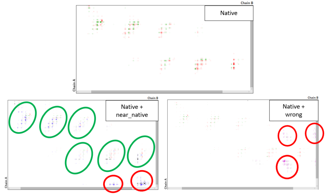
It is important to take into account that here we are accessing to two types of information: which contacts are shared between the two structures and which scores are assigned to these contacts. The "global scores" section only takes into account the contact scores. Therefore, to perform a complete assessment of docking poses is recommendable to take into account the global scores as well as the detail analysis. By doing so, we can differentiate near-native from incorrect docking poses.
Tutorial 4: Assess the effect of a mutation in the stability of a protein-protein interaction
To check the example of this tutorial, click here.
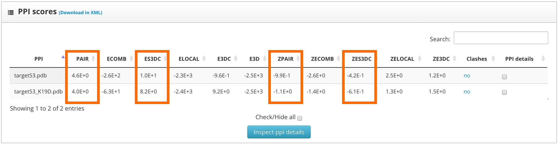
In this tutorial we will work with the structure of docking solutions obtained from the CAPRI scoring dataset, in particular with the target 53. We have obtained an homology model of this structure that contains a mutation using modeller. This mutation is a substitution of a lysine by an aspartate in position 19 of the A chain. The first step is to select the "Protein-protein interactions" option, select a distance for the contact definition and submit a compressed file with the structures under study. In this tutorial we will work with the "CB-CB distance < 12A" option. To access the results page click in "run example".
The results page shows the global scores for the input structures. Check the PAIR, ZPAIR, ES3DC and ZES3DC scores; you can see them highlighted in here:
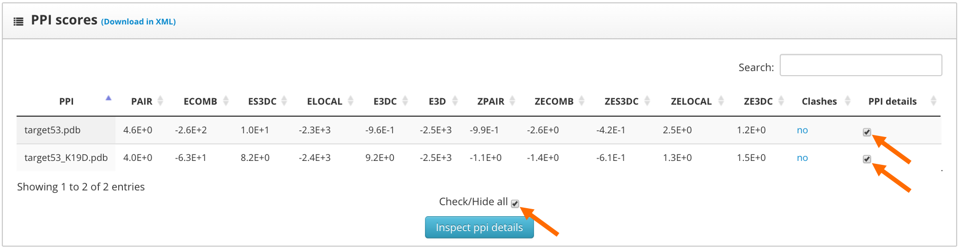
To identify the best folded structures we check for the lowest score in the previously mentioned scoring functions. We see that both structures have similar scores. To perform a more detailed analysis we select the "fold details" option and click into the "inspect fold details" button.
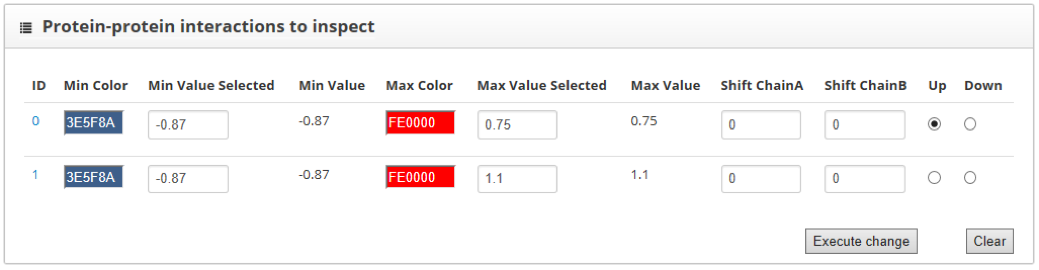
Here we find two sections: "Protein-protein interactions to inspect" and "residue scores". The "Protein-protein interactions to inspect" section allows the assignment of colors to high and low scoring residues. It also allows to shift the protein sequences and to assign the up or down label to each one of the proteins.
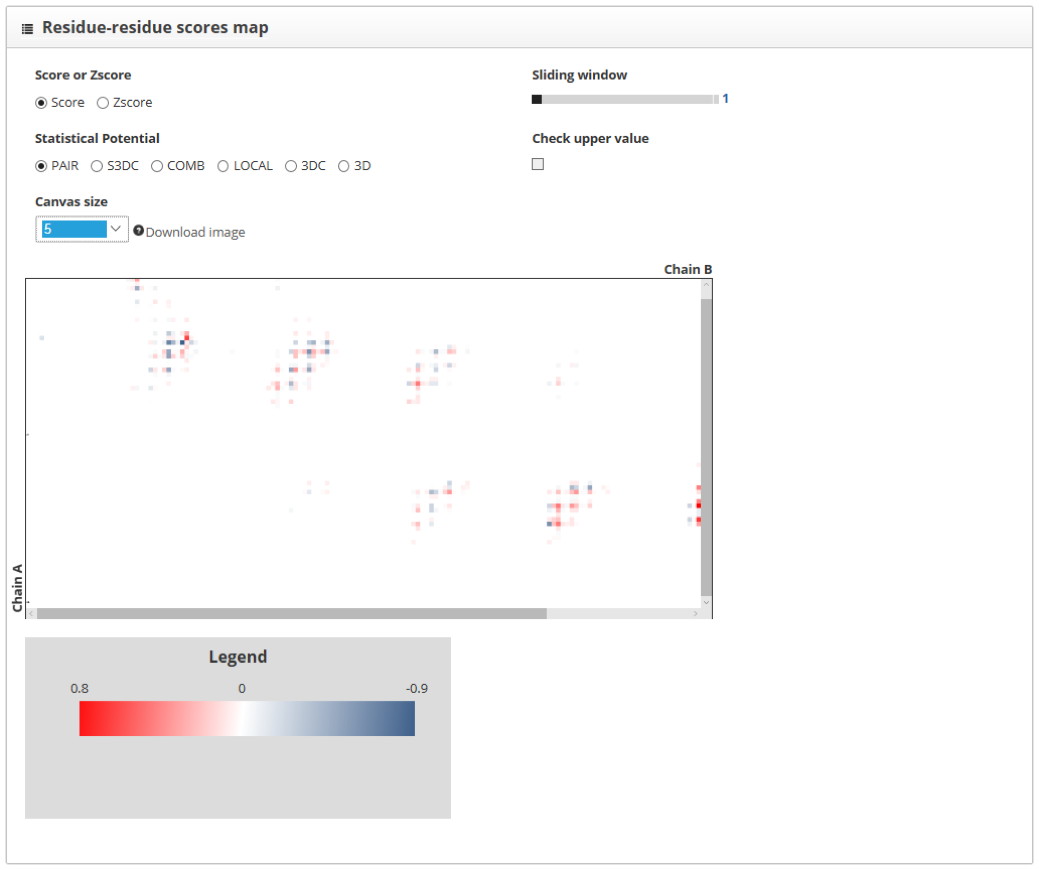
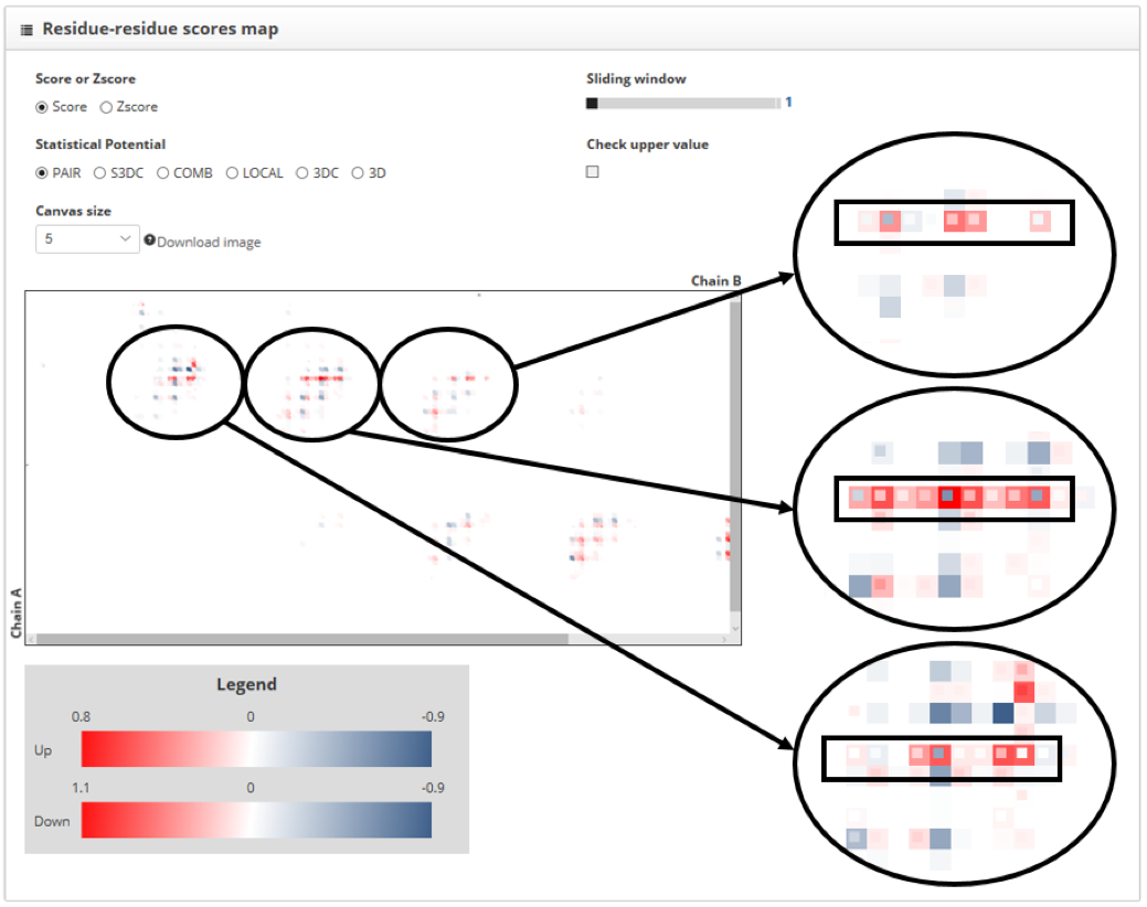
The "residue-residue scores map" section shows the representation from each of the interacting proteins in a different axis. Contacts between the two chains are represented as color dots. The color of these points is informative of whether the contact increases or decreases the stability of the interaction. We can smooth the score map using the "sliding window" tool and increase the size of the map using the "canvas size" option. Besides, the "check upper value" shows the scores for each of the residues of the "up" labeled structure, within the score map.
To compare two PPIs we must assign to them the up or down label in the "Protein-protein interaction to inspect" section. If we increase the size of the score map we will see that protein contacts for the "up" structure are represented with small squares, while the "down" structure ones are represented with big hollow squares. When the same contact is found in both structures, the two squares that represent them fit. In this tutorial we assign the "up" label to the wild type interaction and the "down" to the mutant one.
We can see how the contacts of the two structures overlap almost perfectly. The color of the square is telling us which contacts increase PPI stability and which do not. The color corresponding with the "min color" label in the "protein-protein interactions to inspect" section indicates low scores and high stability, while the one corresponding with "max color" indicates the opposite. We see that in a row of the map, on position 19 for the chain A, the mutant structure is having several contacts that decrease the stability of the interaction. Regions containing contacts for residue 19 from the chain A are shown in detail and highlighted in the next image:
This indicates that, although this mutation has a low impact in the overall score, locally decreases the stability of this protein-protein interaction.